CNR Bioinformatics Workshop
3. Secondary Analysis
We are going to analyze aligned scRNAseq data in R, the most popular language for this type of work at the moment.
3.1 Install R libraries with Miniconda
First, let’s install some packages with conda. Fire up the cmd.
conda activate myEnv
conda install -c conda-forge r-base
conda install -c conda-forge r-seurat
conda install -c conda-forge r-ggplot2
conda install -c conda-forge r-dplyr
3.2 Import R libraries, set working directory and data
library(Seurat)
Attaching SeuratObject

Attaching sp
3.3 Load data
df <- Read10X("./outs/filtered_feature_bc_matrix/")
df0 <- CreateSeuratObject(counts = df,
                         assay = "RNA",
                         project = "hCO",
                         min.cells = 10,
                         min.features = 200)
Warning message:
"Feature names cannot have underscores ('_'), replacing with dashes ('-')"
df0
An object of class Seurat
16527 features across 2342 samples within 1 assay
Active assay: RNA (16527 features, 0 variable features)
df0$percent.mt <- PercentageFeatureSet(df0, pattern = "^MT-")
options(repr.plot.width = 10, repr.plot.height = 5)
VlnPlot(df0,
       log = T,
       pt.size = 0,
       features = c("nFeature_RNA", "nCount_RNA", "percent.mt"))
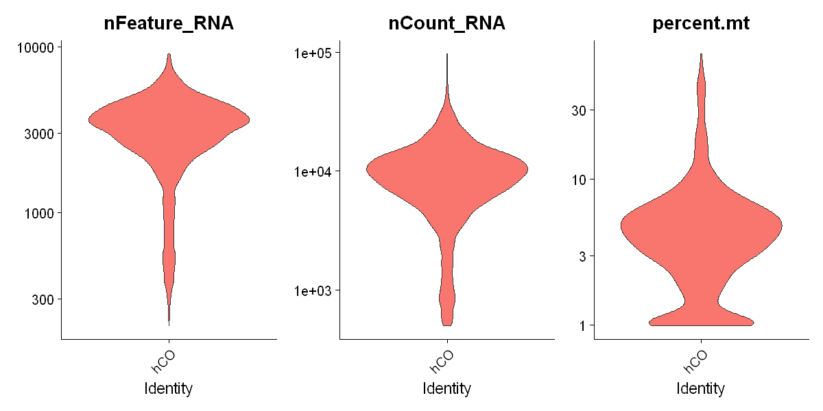
Keep cells with more than 1000 UMI and less than 10% of reads mapped to mitochondrial genome
df0 <- df0[ , df0$nCount_RNA > 1000 & df0$percent.mt < 10]
df0
An object of class Seurat
16527 features across 2125 samples within 1 assay
Active assay: RNA (16527 features, 0 variable features)
Remove mitochondrial genes
MTs <- grep("^MT-", rownames(df0), value = T)
df0 <- df0[!(rownames(df0) %in% MTs)]
df0
An object of class Seurat
16514 features across 2125 samples within 1 assay
Active assay: RNA (16514 features, 0 variable features)
3.4 Normalization between different read depth (total UMI counts) by cell
df0 <- NormalizeData(df0, normalization.method = "LogNormalize", scale.factor = 10000)
3.5 Find highly variable genes
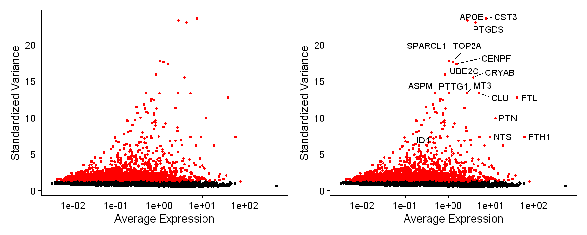
df0 <- FindVariableFeatures(df0, selection.method = "vst", nfeatures = 2000)
hvg <- VariableFeatures(df0)
top50 <- head(VariableFeatures(df0), 50)
options(repr.plot.width = 10, repr.plot.height = 4)
plot1 <- VariableFeaturePlot( df0, log = T )
plot2 <- LabelPoints(plot = plot1, points = top50, repel = TRUE)
plot1 + NoLegend() + plot2 + NoLegend()
When using repel, set xnudge and ynudge to 0 for optimal results

Warning message:
"ggrepel: 29 unlabeled data points (too many overlaps). Consider increasing max.overlaps"
3.6 Scaling data
df0 <- ScaleData(df0, features = hvg)
Centering and scaling data matrix
3.7 Perform principal component analysis
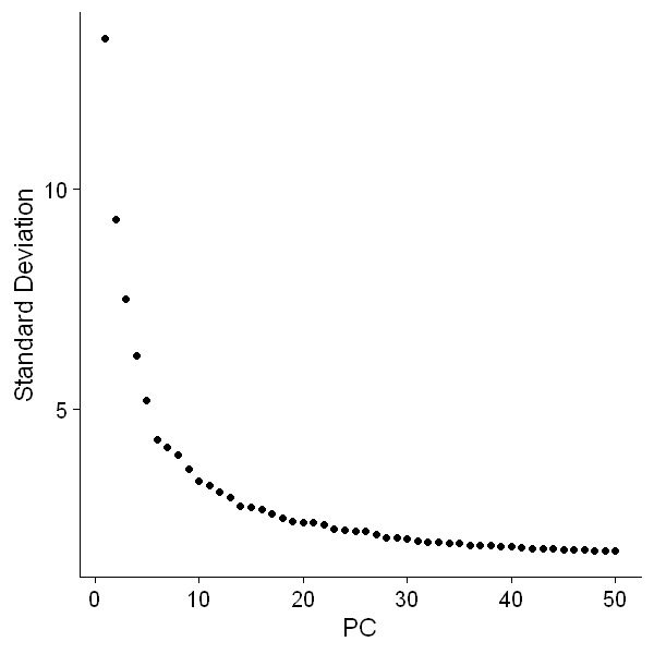
df0 <- RunPCA(df0, npcs = 50, features = hvg, verbose = F)
options(repr.plot.width = 5, repr.plot.height = 5)
ElbowPlot(df0, ndims = 50)
3.8 2D representation with UMAP
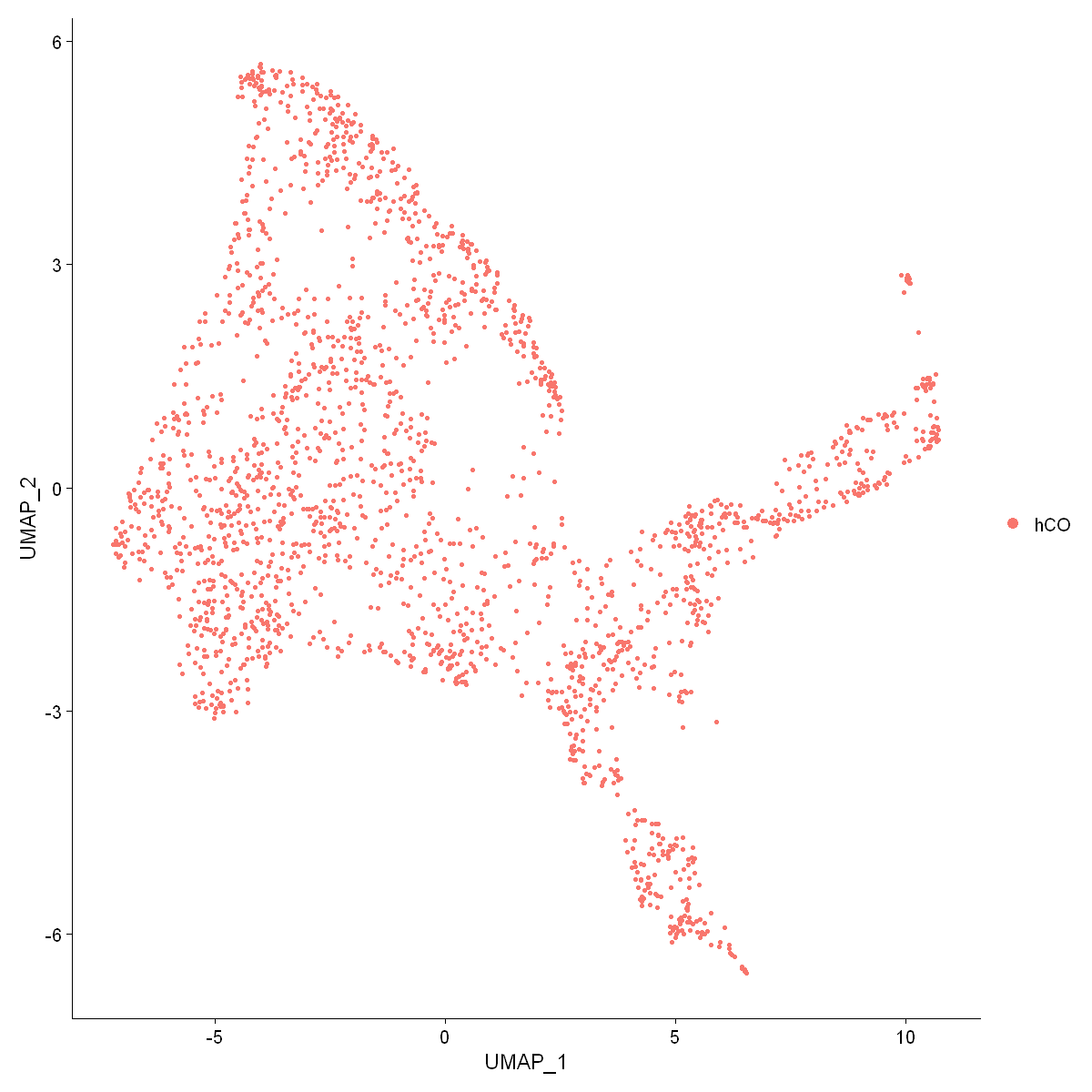
df0 <- RunUMAP(df0, dims = 1:30)
Warning message:
"The default method for RunUMAP has changed from calling Python UMAP via reticulate to the R-native UWOT using the cosine metric
To use Python UMAP via reticulate, set umap.method to 'umap-learn' and metric to 'correlation'
This message will be shown once per session"
11:03:49 UMAP embedding parameters a = 0.9922 b = 1.112

11:03:49 Read 2125 rows and found 30 numeric columns

11:03:49 Using Annoy for neighbor search, n_neighbors = 30

11:03:49 Building Annoy index with metric = cosine, n_trees = 50

0%   10   20   30   40   50   60   70   80   90   100%

[----|----|----|----|----|----|----|----|----|----|

*
*
*
*
*
*
*
*
*
*
*
*
*
*
*
*
*
*
*
*
*
*
*
*
*
*
*
*
*
*
*
*
*
*
*
*
*
*
*
*
*
*
*
*
*
*
*
*
*
*
|

11:03:49 Writing NN index file to temp file C:\Users\ZLI2\AppData\Local\Temp\3\RtmpALR9le\file290435047be8

11:03:49 Searching Annoy index using 1 thread, search_k = 3000

11:03:49 Annoy recall = 100%

11:03:50 Commencing smooth kNN distance calibration using 1 thread

11:03:50 Initializing from normalized Laplacian + noise

11:03:50 Commencing optimization for 500 epochs, with 82866 positive edges

11:03:58 Optimization finished
options(repr.plot.width = 10, repr.plot.height = 10)
DimPlot(df0, pt.size = 1,reduction = "umap")
df0 <- FindNeighbors(df0, reduction = "umap", dims = 1:2)
Computing nearest neighbor graph

Computing SNN
df0 <- FindClusters(df0)
Modularity Optimizer version 1.3.0 by Ludo Waltman and Nees Jan van Eck

Number of nodes: 2125
Number of edges: 44905

Running Louvain algorithm...
Maximum modularity in 10 random starts: 0.9030
Number of communities: 20
Elapsed time: 0 seconds
options(repr.plot.width = 10, repr.plot.height = 10)
DimPlot(df0, label = T, group.by = "seurat_clusters", reduction = "umap")

Adjust resolution to get more or fewer clusters
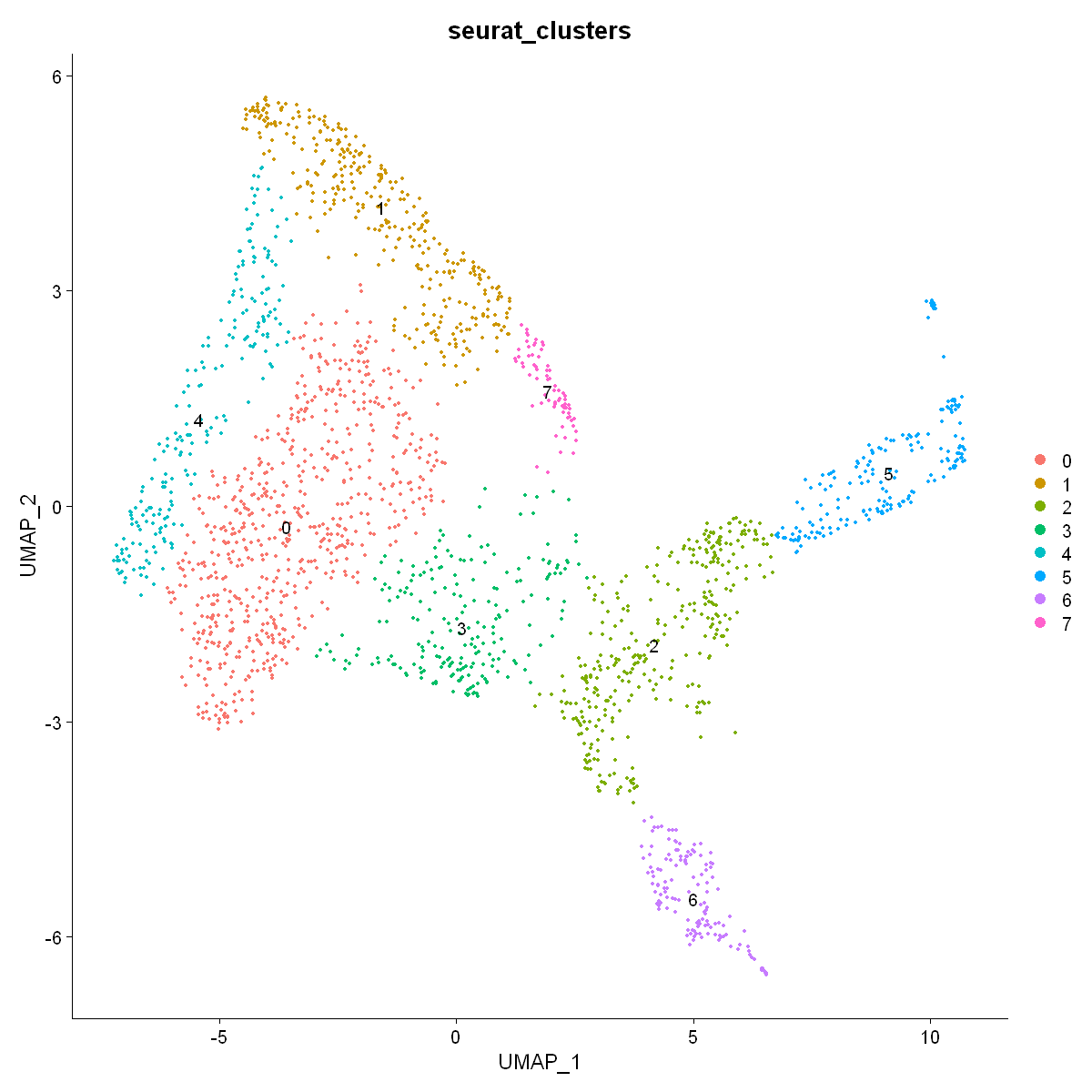
df0 <- FindClusters(df0, resolution = 0.1)
Modularity Optimizer version 1.3.0 by Ludo Waltman and Nees Jan van Eck

Number of nodes: 2125
Number of edges: 44905

Running Louvain algorithm...
Maximum modularity in 10 random starts: 0.9652
Number of communities: 8
Elapsed time: 0 seconds
DimPlot(df0, label = T, group.by = "seurat_clusters", reduction = "umap")
3.9 Differential gene expression analysis
DEX <- FindAllMarkers(df0, only.pos = T)
Calculating cluster 0

For a more efficient implementation of the Wilcoxon Rank Sum Test,
(default method for FindMarkers) please install the limma package
--------------------------------------------
install.packages('BiocManager')
BiocManager::install('limma')
--------------------------------------------
After installation of limma, Seurat will automatically use the more
efficient implementation (no further action necessary).
This message will be shown once per session

Calculating cluster 1

Calculating cluster 2

Calculating cluster 3

Calculating cluster 4

Calculating cluster 5

Calculating cluster 6

Calculating cluster 7
DEX
| p_val | avg_log2FC | pct.1 | pct.2 | p_val_adj | cluster | gene | |
|---|---|---|---|---|---|---|---|
| <dbl> | <dbl> | <dbl> | <dbl> | <dbl> | <fct> | <chr> | |
| THSD7A | 6.045978e-196 | 1.8697358 | 0.936 | 0.344 | 9.984329e-192 | 0 | THSD7A |
| CDH7 | 8.096795e-188 | 1.8878890 | 0.677 | 0.088 | 1.337105e-183 | 0 | CDH7 |
| CADM1 | 9.910354e-165 | 1.4515527 | 0.961 | 0.594 | 1.636596e-160 | 0 | CADM1 |
| NTS | 1.028108e-156 | 2.3811702 | 0.753 | 0.192 | 1.697817e-152 | 0 | NTS |
| LINC00643 | 6.132768e-156 | 1.2198939 | 0.821 | 0.219 | 1.012765e-151 | 0 | LINC00643 |
| CNTNAP2 | 1.002729e-146 | 1.3381175 | 0.975 | 0.578 | 1.655906e-142 | 0 | CNTNAP2 |
| NEUROD6 | 1.564023e-145 | 1.3210439 | 0.994 | 0.573 | 2.582828e-141 | 0 | NEUROD6 |
| BCL11B | 5.386061e-141 | 1.2989753 | 0.950 | 0.489 | 8.894541e-137 | 0 | BCL11B |
| GABRG2 | 1.876424e-133 | 1.1450737 | 0.776 | 0.231 | 3.098726e-129 | 0 | GABRG2 |
| KAZN | 2.155009e-132 | 1.2500493 | 0.857 | 0.385 | 3.558781e-128 | 0 | KAZN |
| GPR22 | 3.700312e-131 | 1.3231371 | 0.771 | 0.219 | 6.110695e-127 | 0 | GPR22 |
| GABRB3 | 1.038149e-130 | 1.2282807 | 0.868 | 0.399 | 1.714400e-126 | 0 | GABRB3 |
| DOK6 | 2.392019e-129 | 1.1933333 | 0.830 | 0.320 | 3.950180e-125 | 0 | DOK6 |
| OPCML | 2.384368e-127 | 0.9593867 | 0.666 | 0.156 | 3.937545e-123 | 0 | OPCML |
| MAP1B | 1.467895e-125 | 0.9586851 | 0.998 | 0.974 | 2.424082e-121 | 0 | MAP1B |
| GUCY1A3 | 4.140991e-125 | 0.9108090 | 0.513 | 0.069 | 6.838433e-121 | 0 | GUCY1A3 |
| CELF4 | 1.823213e-124 | 1.2076658 | 0.896 | 0.418 | 3.010853e-120 | 0 | CELF4 |
| CRYM | 2.752345e-123 | 1.1846565 | 0.703 | 0.171 | 4.545222e-119 | 0 | CRYM |
| PCSK2 | 1.134087e-122 | 0.8380855 | 0.603 | 0.112 | 1.872832e-118 | 0 | PCSK2 |
| PDE1A | 1.246173e-122 | 1.1144271 | 0.941 | 0.428 | 2.057930e-118 | 0 | PDE1A |
| FEZF2 | 7.187010e-121 | 1.1284446 | 0.911 | 0.457 | 1.186863e-116 | 0 | FEZF2 |
| VSNL1 | 1.687290e-120 | 1.3733470 | 0.645 | 0.142 | 2.786390e-116 | 0 | VSNL1 |
| LMO3 | 2.402370e-118 | 1.1753594 | 0.918 | 0.457 | 3.967274e-114 | 0 | LMO3 |
| GRIA2 | 1.041490e-117 | 1.1211322 | 0.967 | 0.518 | 1.719916e-113 | 0 | GRIA2 |
| LPL | 2.722715e-117 | 1.5427983 | 0.742 | 0.284 | 4.496291e-113 | 0 | LPL |
| ENC1 | 6.710271e-116 | 1.3280815 | 0.966 | 0.616 | 1.108134e-111 | 0 | ENC1 |
| BCL11A | 7.457177e-115 | 1.0586476 | 0.981 | 0.682 | 1.231478e-110 | 0 | BCL11A |
| LIN7A | 1.133347e-113 | 0.9562324 | 0.773 | 0.287 | 1.871609e-109 | 0 | LIN7A |
| EDIL3 | 1.759098e-113 | 1.6850054 | 0.655 | 0.203 | 2.904974e-109 | 0 | EDIL3 |
| ADAMTS3 | 7.684031e-113 | 0.7352453 | 0.482 | 0.067 | 1.268941e-108 | 0 | ADAMTS3 |
| ⋮ | ⋮ | ⋮ | ⋮ | ⋮ | ⋮ | ⋮ | ⋮ |
| VEZT1 | 0.006367994 | 0.4544607 | 0.594 | 0.575 | 1 | 7 | VEZT |
| EDF1 | 0.006396941 | 0.2768622 | 0.928 | 0.925 | 1 | 7 | EDF1 |
| CACNB3 | 0.006416318 | 0.3197875 | 0.304 | 0.206 | 1 | 7 | CACNB3 |
| KCTD161 | 0.006477961 | 0.4357945 | 0.246 | 0.146 | 1 | 7 | KCTD16 |
| ZFAND61 | 0.006556065 | 0.3108803 | 0.609 | 0.526 | 1 | 7 | ZFAND6 |
| FDPS2 | 0.006565919 | 0.4212422 | 0.681 | 0.684 | 1 | 7 | FDPS |
| SLC35B4 | 0.006706530 | 0.4090899 | 0.333 | 0.241 | 1 | 7 | SLC35B4 |
| KAT6B1 | 0.006719325 | 0.3702466 | 0.667 | 0.635 | 1 | 7 | KAT6B |
| SECISBP2 | 0.006741026 | 0.4191203 | 0.580 | 0.554 | 1 | 7 | SECISBP2 |
| PPIB2 | 0.006797369 | 0.3360325 | 0.841 | 0.862 | 1 | 7 | PPIB |
| ACAT22 | 0.006837845 | 0.3273365 | 0.594 | 0.505 | 1 | 7 | ACAT2 |
| TM7SF21 | 0.006947730 | 0.3336245 | 0.478 | 0.394 | 1 | 7 | TM7SF2 |
| ASCL12 | 0.007045782 | 0.4827441 | 0.261 | 0.146 | 1 | 7 | ASCL1 |
| FAM129B | 0.007381191 | 0.2510892 | 0.101 | 0.039 | 1 | 7 | FAM129B |
| TOMM22 | 0.007427035 | 0.2621766 | 0.652 | 0.609 | 1 | 7 | TOMM22 |
| FKBP1A | 0.007607480 | 0.3741991 | 0.739 | 0.726 | 1 | 7 | FKBP1A |
| SERINC51 | 0.007875080 | 0.4397336 | 0.333 | 0.232 | 1 | 7 | SERINC5 |
| SRSF22 | 0.007977450 | 0.3277416 | 0.710 | 0.700 | 1 | 7 | SRSF2 |
| FADS11 | 0.008017162 | 0.3882929 | 0.594 | 0.571 | 1 | 7 | FADS1 |
| ZNF931 | 0.008042945 | 0.2557433 | 0.217 | 0.124 | 1 | 7 | ZNF93 |
| HNRNPU1 | 0.008578680 | 0.3404948 | 0.942 | 0.889 | 1 | 7 | HNRNPU |
| UQCRC12 | 0.008897287 | 0.4097974 | 0.594 | 0.567 | 1 | 7 | UQCRC1 |
| ADH53 | 0.009296225 | 0.2925211 | 0.739 | 0.760 | 1 | 7 | ADH5 |
| USP3 | 0.009384821 | 0.3955659 | 0.493 | 0.452 | 1 | 7 | USP3 |
| CHD6 | 0.009613483 | 0.4403142 | 0.478 | 0.410 | 1 | 7 | CHD6 |
| DUBR | 0.009658439 | 0.3439089 | 0.188 | 0.106 | 1 | 7 | DUBR |
| STK17A | 0.009694749 | 0.5527915 | 0.449 | 0.380 | 1 | 7 | STK17A |
| EZH21 | 0.009740367 | 0.2961342 | 0.362 | 0.261 | 1 | 7 | EZH2 |
| COMMD5 | 0.009885292 | 0.3097648 | 0.304 | 0.216 | 1 | 7 | COMMD5 |
| ATP5L | 0.009998582 | 0.2754477 | 0.957 | 0.942 | 1 | 7 | ATP5L |
3.10 Save files
write.csv(DEX, "DEX.csv")
saveRDS(df0, file = "df0.rds")